The first step for the calculation of the earthquake-induced displacement of an embedded cantilever retaining wall is the definition of the net pressure distribution exerted by the soil on the wall. It is worth to point out that the term net pressure is employed to indicate the difference between the passive and active soil stresses on the wall. To this purpose, DReW Seismic refers to the solution provided by Conte, Troncone and Vena (2017). An example of this distribution is shown in the following figure.
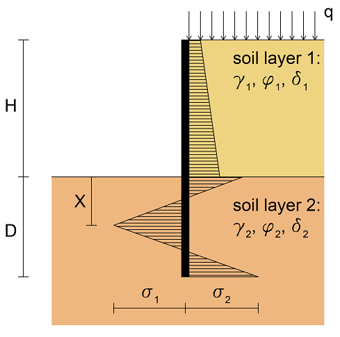
Net pressure distribution acting on the wall
This distribution depends on the seismic horizontal coefficient, kh, which varies during the earthquake. At the generic time t, the seismic horizontal coefficient is related to the ground acceleration a(t) through the following equation kh(t)=a(t)/g, where g is the gravity acceleration.
As the type of movement usually experienced by these structures consists of an approximately rigid rotation around a point located close to the wall base, an active limit state occurs behind the wall, above the excavation level. Below this level, the active pressure and passive resistance are fully mobilized down to a depth X, whereas the passive resistance is not fully mobilized at higher depths. As an approximation, it is assumed that the net pressures varies linearly from σ1 to σ2, as shown from the above figure. More details can be found in the paper by Conte, Troncone and Vena (2017).
The active thrust and passive resistance acting above the depth X depend on the active and passive earth pressure coefficients in seismic conditions, KaE and KpE, respectively. These coefficients are calculated in DReW Seismic using the solution developed by Lancellotta (2007). The depth X and the net pressure at the wall base σ2 are calculated from the equilibrium. Their solution can be found in the paper by Conte, Troncone and Vena (2017).